

The core of the FFD pipeline’s data balancing strategy is a Generative Adversarial Network (GAN) built with TensorFlow/Keras. The GAN is trained exclusively on the 492 real fraudulent transactions, and once converged, its generator produces synthetic fraud samples that are statistically indistinguishable from real ones. These synthetic samples are then merged with the original dataset to create a balanced training set for the downstream classifiers.Documentation Index
Fetch the complete documentation index at: https://mintlify.com/Antisource/FFD/llms.txt
Use this file to discover all available pages before exploring further.
Adversarial Training — Generator vs. Discriminator
The GAN framework pits two neural networks against each other in a minimax game: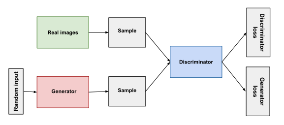
- Generator — Takes a random noise vector as input and tries to produce synthetic fraud feature vectors realistic enough to fool the discriminator.
- Discriminator — Takes a feature vector (either real fraud data or generator output) and tries to correctly classify it as real (
1) or synthetic (0).
FFD requires TensorFlow 2.11. Install it with:Other TensorFlow 2.x versions may work, but 2.11 is the version used during development and testing.
Generator Model
The generator transforms a random noise vector into a synthetic feature vector of the same dimensionality as the real fraud data (29 features).| Layer | Output Shape | Notes |
|---|---|---|
Dense(32) + BatchNormalization | (None, 32) | Entry point; he_uniform initializer; relu activation |
Dense(64) + BatchNormalization | (None, 64) | Expanding representation |
Dense(128) + BatchNormalization | (None, 128) | Peak capacity layer |
Dense(29, linear) | (None, 29) | Output layer; linear activation to match real data range |
- Input: A noise vector of dimension 29 (matching the number of fraud features).
BatchNormalizationafter each hidden layer stabilises training by normalising intermediate activations, preventing vanishing/exploding gradients.- Linear output activation allows the generator to produce values across the full real-number range, matching the PCA-transformed fraud feature distribution.
- Total trainable parameters: 15,581 (16,029 total including BatchNorm non-trainable).
Discriminator Model
The discriminator is a binary classifier that distinguishes real fraud transactions from generator outputs.| Layer | Output Shape | Notes |
|---|---|---|
Dense(32) | (None, 32) | Entry point; he_uniform initializer |
Dense(64) | (None, 64) | Widening hidden layer |
Dense(32) | (None, 32) | Compression |
Dense(32) | (None, 32) | Further refinement |
Dense(16) | (None, 16) | Bottleneck |
Dense(1, sigmoid) | (None, 1) | Binary output: real (≈1) vs. synthetic (≈0) |
- Optimizer: Adam with
binary_crossentropyloss — standard for binary classification. - Sigmoid output produces a probability score, enabling gradient-based feedback to the generator during GAN training.
- Total parameters: 6,753 (all trainable).
Combined GAN
The full GAN is assembled by stacking the generator and a frozen discriminator, so that only the generator’s weights are updated during adversarial training.discriminator.trainable = False— Freezing the discriminator’s weights inside the GAN model is essential. During GAN training, gradients flow back through the discriminator to update only the generator. If the discriminator were allowed to update simultaneously, both networks would chase a moving target and training would destabilise.Input → Generator → Discriminator— The data flow is: random noise → generator produces synthetic features → discriminator scores them. The GAN is trained to push this score toward1(real), incentivising the generator to improve.- GAN compilation uses
optimizer='adam'andloss='binary_crossentropy'. - Combined total parameters: 22,782.
Training Process
Initialise models
Instantiate the generator, discriminator, and combined GAN. Compile the GAN with Adam and binary cross-entropy loss.
Configure training hyperparameters
Set the number of epochs, batch size, and derive the half-batch size used for balanced real/fake training batches.
Adversarial training loop
Each epoch alternates between updating the discriminator on real and fake samples, then updating the generator via the frozen-discriminator GAN.
Monitor with PCA scatter plots
Every 10 epochs,
monitor_generator() projects real and synthetic fraud data to 2D via PCA and renders a scatter plot. Convergence is visible when the two clusters overlap closely.Generator
Learns to map 29-dim noise → realistic fraud features over 1,000 epochs
Discriminator
Binary classifier that drives generator improvement through adversarial loss
Training epochs
1,000 epochs, batch size 64 (half-batch 32 real + 32 fake per discriminator update)
Monitoring
PCA scatter plot every 10 epochs to visualise real vs. synthetic fraud distribution